Nyquist stability criterion is based on the principle of argument which states that if there are P poles and Z zeros of the transfer function enclosed in s-plane contour, then the corresponding GH plane contour will encircle the origin Z-times in the clockwise direction and P-times in anticlockwise direction, i.e. (P−Z) times in anticlockwise direction.
The Routh–Hurwitz criterion and root locus methods are used to determine the stability of the linear single-input single-output (SISO) system by finding the location of the roots of the characteristic equation in s-plane. The Nyquist stability criterion derived by H. Nyquist is a semi-graphical method that helps in determining the absolute stability of the closed-loop system graphically from frequency response of loop transfer function (Nyquist plot) without determining the closed-loop poles. The Nyquist plot of a loop transfer function G(s)H(s) is a graphical representation of the frequency response analysis when the frequency ω is varied from -∞ to ∞. Since most of the linear control systems are analyzed by using their frequency responses, Nyquist plot will be convenient in determining the stability of the system
Table of Contents
Concept of Nyquist stability criterion
To illustrate this let us consider a contour in the s-plane which encloses one zero of G(s) H(s), say s = α1. The remaining poles and zeros are placed in the s-plane outside the contour as shown in given figure below.
For any non-singular point in the s-plane contour, there is a corresponding point G(s) H(s) in the GH-plane contour. Let s follows a prescribed path as shown in the clockwise direction making one circle and returning to its original position. The phasor (s − α1) will cover an angle of −2π while the net angle covered by the other two phasors, namely (s − β1) and (s − α2) is zero. The phasor representing the magnitude of G(s) H(s) in the GH-plane will undergo a net phase change of −2π.
That is, this phasor will encircle the origin once in the clockwise direction as shown in figure (b) below. If the contour in the s-plane encloses two zeros, α1 and α2 in the s-plane, the contour in the GH-plane will encircle the origin two-times. Generalizing this, it can be stated that for each zero of G(s) H(s) in the s-plane enclosed, there is the corresponding encirclement of origin by the contour in the GH-plane once in the clockwise direction.
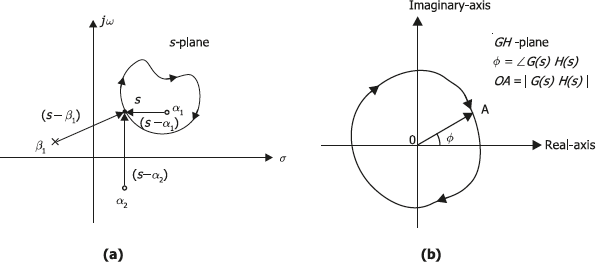
When the contour in the s-plane encloses a pole and a zero say at α and β respectively, both the phasors (s − α) and (s − β) will generate an angle of 2π as s traverses the prescribed path. However since (s − β) will be in the denominator of G(s) H(s), the contour in the GH-plane will experience one clockwise and one counter clockwise encirclement of the origin.
If we have p number of poles and z number of zeros enclosed by the contour in the s-plane, the: contour in the GH-plane will encircle the origin by (p − z) times in counterclockwise direction [since (s − p) is in the denominator of the open loop transfer function, G(s) H(s)].
For a system to be stable, there should not be any zeros of the closed loop transfer function in the right half of s-plane. Therefore, a closed loop system is considered stable, if the number of encirclements of the contour in GH-plane around the origin is equal to the open-loop pole of the transfer function, G(s) H(s).
We can express
G(s) H(s) = [1 + G(s) H(s)] − 1
From this, it can be said that the contour G(s) H(s) in GH-plane corresponding to Nyquist contour in the s-plane is the same as contour of [1 + G(s) H(s)] drawn from the point (−1 + j0).
Thus it can be stated that if the open-loop transfer function G(s) H(s) corresponding to Nyquist contour in the s-plane encircles the point at (−1 + j0) in the counterclockwise direction the number of times equal to the right half s-plane poles of G(s) H(s), it can then be said that the closed-loop control system is stable.
Nyquist Path or Nyquist Contour
The transfer function of a feedback control system is expressed as
\frac{C(s)}{R(s)}=\frac{G(s)}{1+G(s)H(s)}
The denominator is equated to 0 to represent the characteristic equation as
1+G(s)H(s)=0
The study of the stability of the closed-loop system is done by determining whether the characteristic equation has any root in the right half of the s-plane. Or, in other words, we have to determine whether C(s)/R(s) has any pole located in the right half of the s-plane. We use a contour in the s-plane which encloses the whole of the right-hand half of the s-plane. The contour will encircle in the clockwise direction having a radius of infinity. If there is any pole on the jω-axis, these are bypasses with small semicircles taking around them. If the system does not have any pole or zero at the origin or in the jω-axis, the contour is drawn as shown in the below figure (b). A few examples of the application of the Nyquist criterion for stability study will be taken up now.

Advantages of Nyquist Plot
The advantages of Nyquist plot are:
- The Nyquist plot helps in determining the relative stability of the system in addition to the absolute stability of the system.
- It determines the stability of the closed-loop system from the open-loop transfer function without calculating the roots of the characteristic equation.
- The Nyquist plot gives the degree of instability of an unstable system and indicates the ways in which the stability of the system can be improved.
- It gives information related to frequency domain characteristics such as Mr, ωr, BW etc..
- It can easily be applied to systems with a pure time delay that cannot be analyzed using the root locus method or Routh–Hurwitz criterion.
Example:
The open-loop transfer function of a unity feedback control system is given as
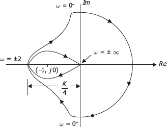
G(s)H(s)=\frac{K}{s(s^{2}+s+4)}Determine the value of K for which the system is stable by applying Nyquist criterion.
Solve:
We have,
G(s)H(s)=\frac{K}{s(s^{2}+s+4)}Putting s=jω, than we get using rationalization,
G(s)H(s)=\frac{-K[\omega +j(4-\omega ^{2})]}{j\omega [(4-\omega ^{2})^{2}+\omega ^{2}]}The crossing of Nyquist plot at the real axis can be found out by equating the imaginary part of the above to 0.
Thus, 4 – ω2 = 0
or, ω = ± 2
The magnitude |G(jω) H(jω)| at ω = ± 2, i.e. at ω2 = 4 is found as
G(s)H(s)=-\frac{K}{4}
The Nyquist plot for G(jω) H(jω) has been drawn as in above figure. From this figure we notice that the intercept on the real axis at ω = ± 2 is -\frac{K}{4}, which is greater than −1.
The value of K is found as
-\frac{K}{4}> -1 \Rightarrow K> 4According to Nyquist stability criterion, if there are P poles and Z zeros in the transfer function enclosed by the s-plane contour, the corresponding contour in the GH-plane must encircle origin Z times in the clockwise direction and P times in the anticlockwise direction resulting encircling (P − Z) times in the anticlockwise direction. Again G(s) H(s) contour around the origin is the same as contour of 1 + G(s) H(s) drawn from (−1 + j0) point on the real axis.
Here the encirclement of −1 + j0 has been in the clockwise direction two times, hence N = −2. There is no pole on the right-hand side of the s-plane and hence P = 0
Putting, P – Z = N,
0 – Z = – 2 or Z = 2
Thus, for K > 4, the system is unstable. The system will be stable if K < 4.