Table of Contents
Concept of Stability
Concept of Stability: A system is said to be stable if it does not exhibit large changes in its output for a small change in its input, initial conditions or its system parameters. In a stable system, the output is predictable and finite for a given input. The definition of stability depends on the type of system. Generally, the stability of a system is classified as stable, unstable and marginally stable.

A linear time-invariant system is said to be stable if the output remains bounded when the system is excited by a bounded input. This is called the Bounded-Input Bounded-Output (BIBO) stability criterion. Further,
- When there is no input, the system should produce a zero output irrespective of initial conditions. This is called the asymptotic stability criterion.
- If a bounded input is applied, the system remains stable for all values of system parameters. This is called absolute stability.
- The stability of a system that exists for a particular range of parameters is called conditional stability.
- The relative stability indicates how close the system is to instability.
- The limitedly stable system produces output that has a constant amplitude of oscillations.
The system can also be classified as Single-Input Single-Output (SISO), Multi-Input Multi-Output (MIMO), linear, nonlinear, time-invariant and time variant systems. In this chapter, the stability of linear SISO time-invariant systems has been discussed.
Definition of stability
An adequate definition of stability with reference to linear control system is given below:
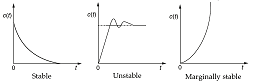
“If any oscillations set up in a system in consequence to application of an input are damped out with respect to time, the system is said to be stable”.
Conversely for unstable systems oscillations are increasing in magnitude. If the magnitude of the oscillation is sustained the system is marginally stable.
Absolute and Relative stability
The term absolute stability is used in relation to qualitative analysis of stability and the term relative stability is used in relation to comparative analysis of stability. The absolute stability can be determined from the location of the roots of the characteristics equation in s-plane. The maximum overshoot, damping ratio and gain margin phase margin are measures for relative stability.
Concept of Stability
Let us consider the following practical example of a ball with different types of surfaces to understand clearly the idea of the stability of a system.

Stable System: A system is said to be stable if it maintains its equilibrium position (original position) when a small disturbance is applied to it. As shown in first figure, even if the ball is disturbed, the equilibrium position will not change. Hence, the system is called asymptotically stable.
Unstable System: A system is said to be unstable if it attains a new equilibrium position that does not resemble the original equilibrium position when a small disturbance is applied to it. As shown in second figure, even if the ball is slightly disturbed, it will upset the equilibrium condition and the ball will roll down from the hill and it will never return back to the equilibrium state. Hence, the system is called unstable.
Marginally Stable System: A system is said to be marginally stable if it attains a new equilibrium position that resembles the original equilibrium position when a small disturbance is applied to it. As shown in the third figure, when an impulsive force is applied, the ball will move for a fixed distance and then stop due to friction. Although the position is changed, the ball will come to a new equilibrium position. Hence, the system is called marginally or non-asymptotically stable.
Oscillatory System: As shown in forth figure, when we apply a disturbing force, the ball will move in both directions (oscillatory motion). Eventually, these oscillations will cease due to the presence of friction and the ball will return back to its stable equilibrium state.
Pole-Zero Location and Conditions for Stability
The transfer function of a single-input, single-output system can be written as
G(s)=\frac{C(s)}{R(s)}= \frac{b_{0}s^{m}+b_{1}s^{m-1}+....+b_{m}}{a_{0}s^{n}+a_{1}s^{n-1}+....+a_{n}}; m< nThe denominator of the transfer function is called characteristic polynomial and its roots are the poles of the transfer function. The characteristic equation is formed by equating the characteristic polynomial to zero. Thus, for the above case, the characteristic equation is
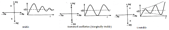
a_{0}s^{n}+a_{1}s^{n-1}+….+a_{n}=0; a_{0}> 0The stability of the closed-loop system can be determined by examining the poles of the closed-loop system, that is, by the roots of the characteristic equation. As we know, the nature of the time response of a system is related to the location of the roots of the characteristic equation in s-plane. For the system to be stable, the roots should have negative real parts. A system will be stable, unstable, or oscillatory depending upon the positions of the roots of the characteristic equation as shown below.
The presence of negativeness of any of the coefficients of the characteristic equation implies that the system is either unstable or at the most has limited stability.
Therefore, the necessary conditions for stability are as follows.
- The positiveness of the coefficients of characteristic equation is necessary. This is the condition for stability of the systems of the first and second order.
- For third and higher-order systems, the positiveness of all the coefficients of the characteristic equation does not ensure the negativeness of the real parts of complex roots. Therefore, it is a necessary but not sufficient condition for the systems of a third and higher-order.
If all the coefficients are positive, the possibility of stability of the system exists.
Methods for Determining the Stability of the System
When the characteristic equation of the system has known parameters, it is very easy to determine the stability of the system by finding the roots of characteristic equation. But when there are some unknown parameters in the equation, the stability of the system can be determined by using the methods given below.
- Routh–Hurwitz Criterion: Routh–Hurwitz criterion was developed independently by E. J. Routh (1892) in the United States of America and A. Hurwitz (1895) in Germany, which is useful to determine the stability of the system without solving the characteristic equation. This is an algebraic method that provides stability information of the system that has the characteristic equation with constant coefficients. It indicates the number of roots of the characteristic equation, which lie on the imaginary axis and in the left half and right half of the s-plane without solving it.
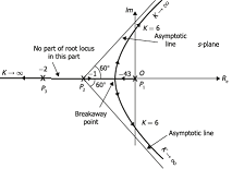
- Root Locus Technique: The technique which was first introduced by W. R. Evans in 1946 for determining the trajectories of the roots of the characteristic equation is known as the root-locus technique. Root locus technique is also used for analyzing the stability of the system with a variation of gain of the system.
- Bode Plot: This is a plot of the magnitude of the transfer function in decibel versus ω and the phase angle versus
 , as is varied from zero to infinity. By observing the behaviour of the plots, the stability of the system is determined.
 - Polar Plot: It provides the magnitude and phase relationship between the input and output response of the system, i.e., a plot of magnitude versus phase angle in the polar coordinates. The magnitude and phase angle of the output response is obtained from the steady-state response of a system on a complex plane when it is subjected to sinusoidal input.
- Nyquist Criterion: This is a semi-graphical method that gives the difference between the number of poles and zeros of the closed-loop transfer function of the system, which are in the right half of the s-plane.
you may also know about State Space Analysis