State Space Analysis

State Space Analysis: The Transfer function approach used to study the behavior of linear time-invariant (LTI) control systems use the time domain or frequency domain methods. In these methods, the systems are modeled using the transfer function approach, which is the ratio of Laplace transform of output to input, neglecting all the initial conditions. Thus this conventional analysis faces all the limitations associated with the transfer function approach. Some of its limitations can be stated as:

1. Naturally, significant initial conditions in obtaining the precise solutions of any system, lose their importance in the conventional approach.
2.  The method is insufficient and troublesome to give a complete time-domain solution of higher-order systems.
3. The transfer function is not very much convenient for the analysis of Multiple Input Multiple Output systems.
4. It gives an analysis of the system for some specific types of inputs like Step, Ramp, etc.
5. It is only applicable to Linear Time-Invariant Systems.
6. The classical methods like Root locus, Bode plot, etc. are basically trial and error procedures that fail to give the optimal solution required.

Hence it is absolutely necessary to use a method of analyzing systems that overcome most of the above-said difficulties. The modern method discussed in this post uses the concept of the total internal state of the system considering all initial conditions. This technique which uses the concept of state is called State Variable Analysis or State Space Analysis. It is essentially a time-domain approach but it has a number of advantages compared to conventional methods of analysis.

Concepts of State, State Variables and State Model

Initially define the concepts of state, state vector, and state-space before proceeding for modeling in state space.

1. State: The state of a dynamic system is the smallest set of variables (called state variables) such that the knowledge of these variables at t = t₀ together with the knowledge of the inputs for t ≥ t₀, completely determines the behavior of the system for t ≥ t₀.

2.State Variables: The state variables of a dynamic system are the smallest set of variables that completely determines the state of the dynamic system.

3. State Vector: This is a vector consisting of n number of state variables that completely determine the behavior of a dynamic system.

4. State Space: The state space is an n-dimensional space whose coordinate axes are the n number of state variables that completely determine the behavior of a dynamic system. Any state can be represented by a point in the state space.

If x₁, x₂,………..x_n are the n state variables of a dynamic system, then its state vector (X) is written by an n x₁, matrix as follows.

X=\begin{bmatrix} x_{1}\\ x_{2}\\ :\\ :\\ x_{n} \end{bmatrix}

where x₁, x₂,……………., x_n all are functions of time t.

5. State Space Equations: The input variables, output variables, and state variables are the three types of variables used in state-space modeling of dynamic systems.

Block Diagram and SFG of a Continuous State-Space Model

The basic element for drawing the block diagram from the state-space model of a system is the integrator. The procedure to obtain the block diagram of a state-space model is given below:

Step 1: The state-space model of a system is obtained by using one of the methods which is to be discussed in the following sections.

Step 2: The individual state equation and output equation are written by using the obtained state-space model.

Step 3: The block diagrams for the individual state equation and output equation are drawn.

Step 4: The number of integrators used for the given state-space model is n (order of matrix A).

Step 5: The individual block diagrams obtained in Step 3 can be interconnected in an appropriate way and by using the n integrators, the block diagram for the given ­state-space model can be obtained.

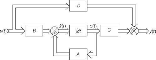
The schematic illustration of a system given by equations \dot{x}(t)=Ax(t)+Bu(t) and y(t)=Cx(t)+Du(t) is shown in figure below. The double lines indicate a multiple-variable signal flow path. The blocks represent matrix multiplication of the vectors and matrices.

Step 6: Once the block diagram of the state-space model is obtained using the steps mentioned in the Signal Flow Graph post, the SFG for the model can be obtained.

State-Space Model Representation for Electric Circuits

The state-space model representation of an electric circuit is done as follows:

Step 1: For a given electric circuit, there exists p number of state variables and q number of output variables.

Step 2: Determine the number of input signals m for a system.

Step 3: If the state variables n and the output variables k are given for an electric circuit, then these variables are assumed as the state variables and output variables. Otherwise, n number of state variables 1˂ n≤ p and k number of output variables, 1˂ k ≤ q are assumed.

Step 4: Using Kirchhoff’s current and/or voltage laws, obtain the differential equation of a system.

Step 5: Using the chosen state variables, the differential equations of a system obtained in the previous step are modified to obtain its first-order derivatives.

Step 6: Determine m number of output equations relating n number of state variables.

Step 7: Finally, by defining the matrices, the state-space model of the electrical circuit is obtained.

Advantages of State-Variable Analysis                                 

The advantages of state-variable analysis are:                                   

1. The state-variable analysis includes the effect of all initial conditions.                                 
2. It is useful to determine the time-domain response of non-linear systems effectively.         
3. State equations involving matrix algebra are highly compatible with simulation on digital computers.
4. It simplifies the mathematical representation of a system.
5. MIMO systems can be easily represented and analyzed using state variables.                                 
6. The simulation diagram for an equation can be obtained directly.
7. Any type of the input can be considered for designing the system.
8. The state variables selected need not necessarily be the physical quantities of the system.