Bode Plot

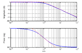
The Bode plot is a frequency response plot of the sinusoidal transfer function of a system. A Bode plot consists of two graphs. One is a plot of the magnitude of a sinusoidal transfer function versus log ω. The other is a plot of the phase angle of a sinusoidal transfer function versus log ω.

The Bode plot can be drawn for both open-loop and closed-loop systems. Usually, the bode plot is drawn for open-loop system. The standard representation of the logarithmic magnitude of open-loop transfer function of G(jω) is 20 log |G(jω)| where the base of the logarithmic is 10. The unit used in this representation of the magnitude is the decibel, usually abbreviated as dB. The curves are drawn on semilog paper, using the log scale (abscissa) for frequency and the linear scale (ordinate) for either magnitude (in decibels) or phase angle (in degrees).

You may also know about Routh-Hurwitz Stability criterion or Root Locus Technique

Magnitude Plot

The magnitude can be expressed in its logarithmic values by finding out the value 20 log₁₀ |G(jω)|, which has a unit as decibel denoted by dB.

For Bode plot    |G(jω)|= 20 log₁₀ |G(jω)| dB.

Phase Angle plot

In this, angle of G(jω) is to be expressed in degrees which is to be plotted against Log ω.

As for both plots X-axis is Log ω both may be drawn on same paper with common X-axis.

Logarithmic Scales (Semilog Papers)

 To sketch the magnitude in dB and phase angle in degrees against Log ω, the logarithmic scale is used. This is available on semilog graph paper. In such paper the X-axis is divided into a logarithmic scale which is non linear one. While Y-axis is divided into linear scale and hence it is called semilog paper.

The interesting part about X-axis is the distance between 1 and 2 is greater than the distance between 2 and 3 and so on. Similarly, on such scale distance between 1 and 10 is equal to the distance between 10 and 100 or between 100 and 1000 and so on. This distance is called 1 decade.

This is because Log 1 = 0 and Log 10 = 1. The distance is 1 decade which is divided into 10 parts according to logarithmic scale i.e. Log 2, Log 3, ……

 Now Log 10 = 1 and Log 100 = 2. The distance is again (2 – 1) i.e. 1 decade same as between Log 1 and Log 10, further divided into parts as Log 20, Log 30,……

So X-axis is available, which is divided into two, three, or four such cycles i.e. decades.

So it is not necessary to find logarithmic value of ω while plotting on X-axis but the logarithmic scale available takes care of logarithmic value of ω. The advantage of the scale is wide range of frequencies can be accommodated on a single paper.

As Log 0 =  – ∞ it is obvious that X-axis cannot be calibrated from 0 but as per requirement the smallest frequency may be selected as starting frequency like 0.01, 0.1 etc. This hardly affects the result of the frequency response.

The Y axis is divided into linear scale similar to standard graph paper.

The main advantage using the logarithmic representation is that the multiplication and division of magnitudes get replaced by the addition and subtraction respectively.

Procedure for Plotting Bode Plot

Step 1: Put the transfer function in the time constant form.

Step 2: Obtain the comer frequencies of zeros and poles.

Step 3: Low frequency plot can be obtained by considering the term \frac{K}{j\omega ^{r}}, Mark the point 20 log K at ω= 1. Draw a line with slope -20 r db/dec until the first comer frequency (due to a pole or zero) is encountered. If the first comer frequency is due to a zero of order m, change the slope of the plot by + 20 m db/dec at this comer frequency. If the comer frequency is due to a pole, the slope changes by – 20 m db/dec.

Step 4: Draw the line with new slope until the next comer frequency is encountered.

Step 5: Repeat steps 3 and 4 until all comer frequencies are considered. If a complex conjugate pole is encountered the slope changes by – 40 db/dec at ω= ω_n.

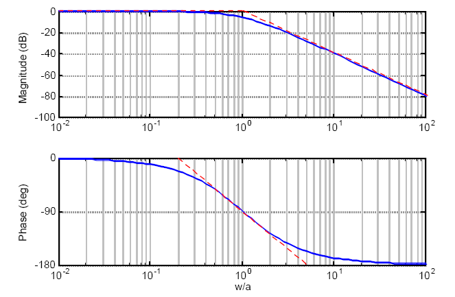
Step 6: To obtain the exact plot, corrections have to be applied at all the comer frequencies and one octave above and one octave below the comer frequencies. To do this, tabulate the errors at various comer frequencies and one octave above and one octave below the comer frequencies. Mark all these points and draw a smooth curve. .

Step 7: The phase angle contributed at various frequencies by individual poles and zeros are tabulated and the resultant angle is found. The angle Vs, frequency is plotted to get a phase angle plot.

Corner frequency

The frequency at which two asymptotes meet is called corner frequency or break frequency. In this case, the corner frequency is at \omega =\frac{1}{T}. The corner frequency divides the frequency response curve of the system as low-frequency region and high-frequency region.

Initial slope and intersection with 0 dB axis for different types of systems.

Type of System (N)	Initial Slope (−20N) dB/dec	Intersection with 0 dB Axis at
Type 0	0 dB/decade	Parallel to 0 dB axis
Type 1	−20 dB/decade	ω = K
Type 2	–40 dB/decade	\omega =\sqrt{K}
Type 3	–60 dB/decade	\omega =K^{1/3}
Type N	−20 N dB/decade	\omega =K^{1/N}

Advantages of Bode Plot                              

The advantages of using Bode plot in plotting the frequency response of a system are:                              

1. Expansion of frequency range of a system is simple.                        
2. Experimental determination of transfer function of a system is simpler if the frequency response of the system is shown using Bode plot.                              
3. Usage of asymptotic straight lines for approximating the frequency response of the system.          
4. Bode plot can be plotted for complicated systems.               
5. Relative stability of the closed-loop system can be analysed by plotting the frequency response of the loop transfer function of the system using Bode plot.                  
6. Frequency domain specifications such as gain crossover frequency, phase crossover frequency, gain margin and phase margin can easily be determined.              
7. The variation of frequency domain specifications can easily be viewed when a controller is added to the existing system.                      
8. The system gain K can be designed based on the required gain and phase margins.
9. Polar plot and Nyquist plot can be constructed based on the data obtained from Bode plot.                                                                      

Disadvantages of Bode Plot                          

The disadvantages of using Bode plot in plotting the frequency response of a system are: 

1. Using Bode plot, it is possible only to determine the absolute and relative stability of the minimum phase system.           
2. Corrections are to be made in the obtained plot to meet the desired frequency plot.